This post is a continuation of my series of posts on the now extremely expired Kaggle competition What’s Cooking. In my previous posts, Data Exploration Part 1 and Data Exploration Part 2, I covered my general strategy of creating the training set from the raw data - TLDR version, I used some text mining techniques to tokenize the ingredients and create a pseudo TFIDF weighting for each ingredient, allowing me to select the terms that are most unique to each cuisine; from these terms, I created a dummy matrix of ingredients, where each row represents a recipe and each column represents a ingredient token.

The goal of this competition is to predict a recipe’s cuisine type based on the ingredients present in the recipe. With a test matrix in hand, lets get to modeling!

In my opinion, the best place to start this modeling process is to try out an ensembled tree method, specifically random forest. Ensembled trees are a great fit for this type of problem as they natively handle multiclass predictions and can be provided a large amount of predictors while remaining robust to overfitting. In this example I’ll be using Random Forest, but boosted methods such as XGboost would be a great choice as well.

At its core, a random forest model is a collection of decision trees given slightly different build information adn parameters being combined to form a model that is typically more predictive than possible with a single tree. I won’t go into the details on the model in this post, but if you’re curious (or just want a refresher) - I like the description in this link. The implementation of a random forest in R is very straightforward:

rf = randomForest(x = train_test$train_dt_x,
                  y = train_test$train_dt_y,
                  ntree = 1500,
                  mtry = 10)

In the above code, x is the training matrix [18626,71], y is the training target a 1 dimensional vector [18626], ntree is the number of decision trees that will be created and ensembled together, mtry is the number of predictors the tree will be given to use for each split, keeping mtry lowish ensures that your trees don’t all look the same (what would be the point of creating a tree monoculture) - not giving it a high enough value ties the hands of your model, not allowing it to perform at the best possible level - in a future post we’ll go into how we can use cross validation to choose the optimal mtry :D.

This model takes a minute or two to run on my machine, but produces a pretty good starting accuracy of 93% and a balanced accuracy of 76% on the held back test data. The balanced accuracy is just the average of recall for each group. I like the balanced accuracy metric best for evaluating this model as it takes into account that the model could have (and does have) varied performance for the different classes.
Calculating these metrics in R is pretty easy with the help of the caret package:

predictions = predict(rf,train_test$test_dt_x)

confusion_calc = caret::confusionMatrix(data = predictions,
                                        reference = train_test$test_dt_y)
all_recall = confusion_calc$byClass[,'Sensitivity']
accuracy = confusion_calc$overall['Accuracy']
balanced_accuracy = mean(all_recall)
}

And we can easily visualize the group accuracy with the following plot rendered by ggplot2:

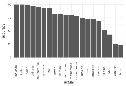
In the next post, I’ll look into strategies to improve our model performance by dealing with the class imbalance!