While super late to the game, the kaggle competition What’s Cooking sounded too fun to miss. The premise is simple - can you design a model to predict a recipe’s cuisine type based on the ingredients present in the recipe? Intuitively, most people would guess that buttermilk + grits + collard greens would be southern American cuisine - but teaching a model that could be tricky - there are 6714 unique ingredients in the dataset, with almost 11 ingredients on average per recipe! I’ll be focusing on the data prep and cleaning in this post, see the full repo here!

For the data cleaning process, I’m going to use R - this could be done in python - but I really like the flexibility and speed of the data.table package. After reading this data into R, you’ll notice the data has the ingredients stored as a vector - which is a pretty inaccessible form for ML. By using the few lines below you can split each ingredient out, making a long version of the data.

train_data = train_data[,lapply(.SD,function(x){unlist(x)}),
                        .SDcols = 'ingredients',
                        by = .(id, cuisine)]

Once the data is in the long shape, its much more simple to work with. Using the data.table package, I can make quick work of some summary statistics:

train_data_recipe_sum = train_data[,.(count_ingredients = .N), by = .(id, cuisine)]

train_data_cuisine_sum = train_data_recipe_sum[,.(frequency = uniqueN(id),
                                                  avg_ingredients = mean(count_ingredients),
                                                  median_ingredients = as.double(median(count_ingredients))), by = .(cuisine)]
train_data_cuisine_sum[,cuisine := factor(cuisine,
                                          levels = train_data_cuisine_sum$cuisine[order(-train_data_cuisine_sum$frequency)])]

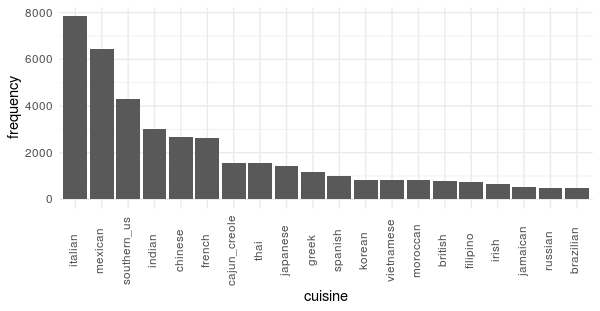
cuisine_freq_plot = ggplot(data = train_data_cuisine_sum, aes(x = cuisine, y = frequency)) + 
  geom_bar(stat = 'identity') + 
  theme_minimal() +
  theme(axis.text.x=element_text(angle=90, vjust = .2))
  

You may be curious about why I had to wrap as.double() around the median() calculation - if so check out this link to a stack overflow post about how data.table’s strong type enforcement clashes with the default behavior of the base::median function - TLDR - median() will preserve the type of the data sent to it– unless that data is a logical or integer class of even length - which makes data.table throw an error.

One of the first things I noticed about this dataset is that the cuisine type classifications are very imbalanced. Italian and Mexican cuisine have 8K and 6.5K recipes while less popular cuisines such as Russian and Brazilian have around 500. This high class imbalance will make prediction difficult - as the most efficient model is to predict that every recipe you see is Italian! In fact, if you knew nothing about the recipe and guessed Italian you’d have a 1 in 5 chance of being right - not bad. As we move forward with modelling we will have to keep this factor in mind.

On average, most recipes have about 10 ingredients, but this varies some by cuisine - for example Moroccan cuisine has the most on average with almost 13 and Japanese has the least with 9. The number of distinct ingredients in this dataset is a bit daunting -6714- and attempting to train a model with all of the ingredients as predictive terms would create an exceptionally wide training matrix with almost as many predictive terms as there are observations! While it is possible to train with that many predictors, in practice, it is usually better to do some feature engineering first to reduce the dimensionality.

To start this process - lets look at which ingredients are the most common:

train_data_ingredient_sum = train_data[,.(frequency = .N), by = .(ingredients)]

train_data_ingredient_sum[,ingredients := factor(ingredients,
                                             levels = train_data_ingredient_sum$ingredients[order(-train_data_ingredient_sum$frequency)])]

setorder(train_data_ingredient_sum,-frequency)

ingredient_freq_plot = ggplot(data = train_data_ingredient_sum[1:10], 
                              aes(x = ingredients, y = frequency)) + 
  geom_bar(stat = 'identity') + 
  theme_minimal() +
  theme(axis.text.x=element_text(angle=90,
                                 vjust = .2)) 

ingredient_freq_plot
  

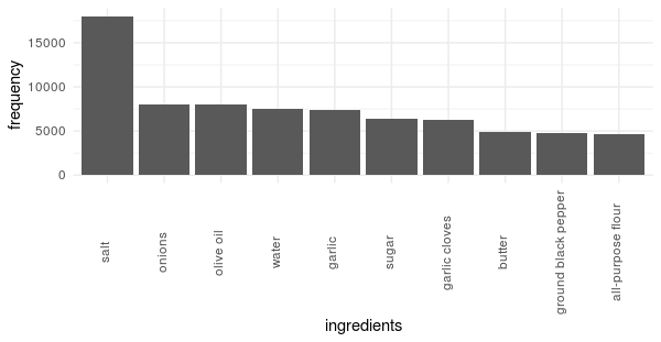
The plot is about as surprising as it is useful for this analysis - most recipes use salt, onions, garlic, and fat. While in some cases it would make sense to retain these dimensions, in this case, knowing that salt is an ingredient would not help the model determine the cuisine type as it is so ubiquitous.

In the next post I’ll go into how I tackled the dimensionality reduction problem by treating the ingredients much like how you treat a corpus of text in a text analytics problem!